A very common problem that arises in both Statistics and Operational Research is optimizing some function of multiple variables, aiming to either maximize or minimise it's value. Often these variables represent certain decisions and the function gives a comparative measure of the quality of this decision. Typically we cannot pick any combination of the variables and have some constraints that must hold, restricting our choices. In this blog post I present a simple fictitious example of an optimisation problem, before going on to discuss some more complex problems which are studied.

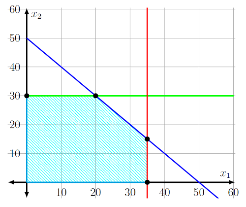
Here the red and the green line represent the upper bounds for the purchase of the apples and pears respectively, due to the constraints of the supplier. Whilst the blue line represents the capacity constraints. The shaded region thus contains all possible choices for \((x_1,x_2)\), this is known as the feasible region. To maximise profit we want to have as high a value of \(x_1\) and \(x_2\) as possible, favoring the latter since it has a higher PPF. This logically leads to an optimal value of \((20,30)\), highlighted by one of the black dots in the diagram. Therefore Claire should buy 20 thousand apples and 30 thousand pears, making her a tidy profit of £40,000 (less the commission for our consultancy services).
More often the methodology is applied to highly complex problems where both the number of variables \(x_i\) and the number of constraints is very large. Examples include network flow problems, seen in my previous post. In such cases, looking at a plot doesn't make much sense, so algorithmic approaches are taken. For example, a famous algorithm for solving linear programs is the Simplex Algorithm, proposed by George Dantzig in 1947.
Even with many variables and constraints, linear programs can still be too simplistic to solve some problems. For example, they only allow continuous variables, whilst many decisions involve binary choices, e.g. yes or no, or integer choices, e.g. if Claire weren't allowed to buy/sell a fraction of a fruit. If we relax the set up of linear programs such that the decisions variables \(x_i\) can be either continuous or integer then we get the class of Mixed Integer Linear Programs (MILPs). These are much more difficult to solve.
A further assumption was the objective function and the constraints are linear functions, which is quite restrictive. In many situations the functions we are dealing with can be quite complex, for example, the objective function for a two-dimensional problem may look something like the plot below. Pretty horrifying.
This leads to an alternative extension, allowing the objective function and/or the constraints to be non-linear functions of the \(x_i\). These functions are usually restricted to be twice differentiable, though this still includes a vast array of functions, such as all finite degree polynomials like the one plotted above. As you might have guessed, these are refereed to as Non-Linear Programs (NLPs).
Both of these classes are brought together, i.e. letting the \(x_i\) be continuous or integer and letting the objective and/or the constrains be non-linear functions of the \(x_i\), into the very general class of Mixed-Integer Non-Linear Programs (MINLPs); a bit of a mouthful. These are very difficult problems to solve and work is still being done today to develop efficient algorithmic procedures for finding optimal solutions.
 A very common problem that arises in both Statistics and Operational Research is optimizing some function of multiple variables, aiming to either maximize or minimise it's value. Often these variables represent certain decisions and the function gives a comparative measure of the quality of this decision. Typically we cannot pick any combination of the variables and have some constraints that must hold, restricting our choices. In this blog post I present a simple fictitious example of an optimisation problem, before going on to discuss some more complex problems which are studied.
Claire's Apples and Pears

Claire owns a business, which sells apples and pears at a food market. Her simple but effective business model ensures that every apple/pear she buys from her supplier is guaranteed to sell, producing a fixed profit per fruit (PPF); 50p for apples and £1 for pears. Thankfully, she is in a situation where she can buy/sell fractions of a fruit, where the price in both situations is just the appropriate proportion of the full price. She is about to make another order from her supplier and wants to know how many apples/pears to buy.
In the presence of such an arbitrage opportunity the obvious thing for Claire to do is buy as many apples and pears as she can. However, there are constraints which must be considered. The supplier has an upper limit on the amount of each fruit Claire can purchase per order; 35 thousand apples and 30 thousand pears. Further, Claire has to store them all in her shed, which does unfortunately have a capacity, at the value of 50 thousand apples/pears (its quite a big shed).
This is an optimisation problem. Specifically, a mathematical programming problem, in which we are aiming to maximise Claire's profits, whilst satisfying the supplier and capacity constraints. To formulate the problem mathematically we need to introduce some variables which can represent possible choices for the order.
Let \(x_1\) denote the number of apples, whilst \(x_2\) represents the number of pears, so that \((x_1, x_2)\) represents a possible order. In mathematical programming these \(x_i\) are referred to as the decision variables. The function we are maximising is \(f(x_1, x_2) = 0.5x_1 + x_2\), representing the profit given a choice of decision variables. This is usually referred to as the objective function. The problem can now be written as follows
\(\text{maximize} \quad 0.5x_1 + x_2 \)
\(\text{subject to} \quad x_1 + x_2 \leq 50\)
\( 0 \leq x_1 \leq 35\)
\(0 \leq x_2 \leq 30\)
Since we have just two variables it is possible to plot the set of pairs \((x_1, x_2)\) which satisfy the above constraints, see the diagram of this below.
Life's Hard
Claire's problem was a very simple example of a linear program (LP), since the objective function and the constraints were linear functions of the \(x_i\). Though this serves as a good illustration of the approach, its highly unlikely that mathematical programming will be used to solve such problems. Common sense tends to deal with these.More often the methodology is applied to highly complex problems where both the number of variables \(x_i\) and the number of constraints is very large. Examples include network flow problems, seen in my previous post. In such cases, looking at a plot doesn't make much sense, so algorithmic approaches are taken. For example, a famous algorithm for solving linear programs is the Simplex Algorithm, proposed by George Dantzig in 1947.
Even with many variables and constraints, linear programs can still be too simplistic to solve some problems. For example, they only allow continuous variables, whilst many decisions involve binary choices, e.g. yes or no, or integer choices, e.g. if Claire weren't allowed to buy/sell a fraction of a fruit. If we relax the set up of linear programs such that the decisions variables \(x_i\) can be either continuous or integer then we get the class of Mixed Integer Linear Programs (MILPs). These are much more difficult to solve.
A further assumption was the objective function and the constraints are linear functions, which is quite restrictive. In many situations the functions we are dealing with can be quite complex, for example, the objective function for a two-dimensional problem may look something like the plot below. Pretty horrifying.
 |
| \(f(x_1, x_2) = 4x_1^2-2.1x_1^4+\frac{1}{3}x_1^6+x_1x_2-4x_2^2+4x_2^4\) |
This leads to an alternative extension, allowing the objective function and/or the constraints to be non-linear functions of the \(x_i\). These functions are usually restricted to be twice differentiable, though this still includes a vast array of functions, such as all finite degree polynomials like the one plotted above. As you might have guessed, these are refereed to as Non-Linear Programs (NLPs).
Both of these classes are brought together, i.e. letting the \(x_i\) be continuous or integer and letting the objective and/or the constrains be non-linear functions of the \(x_i\), into the very general class of Mixed-Integer Non-Linear Programs (MINLPs); a bit of a mouthful. These are very difficult problems to solve and work is still being done today to develop efficient algorithmic procedures for finding optimal solutions.
Comments
Post a Comment